SIEVE IR v1.0 Retrospective
Written: , Published: , Author: Kimberlee Model, Tags: SIEVE IR, Retrospective, v1.0.1, outdated,
In our previous post we took a first look at the SIEVE IR, presenting it as impartially as possible. Today we will take a more "opinionated" or normative look at the IR. On the one hand, we are very proud of this accomplishment — (to our knowledge) the first widely implemented circuit representation for ZK. However, we’d also like to acknowledge that the IR has its flaws and highlight where we think there is room for improvement.
If you understood the previous introduction post, then you should be in a good position to read this one too.
What Did We Get Right?
Looking at the goals we set out for the IR, here’s where we think it is a success.
- Backend Interoperability
-
The IR is successfully integrated with every ZK backend in the SIEVE program. This means that so long as two backends can share the same prime, they can prove the same witnessed statement. The T&E Team was even able to use the SIEVE profile of zkInterface to convert from the IR to R1CS and use
libsnarkas a testing baseline. - Succinct Relations
-
The IR enables a relatively short relation to expand into a far "longer" (at least in gate count) proof. This means that a given relation in the IR may be far shorter than its equivalent in, say, Bristol Fashion or R1CS.
- Interoperable Text and Binary
-
This is sort of an odd-ball feature of the IR, but from the start we realized that an IR has two potentially conflicting goals: On the one hand, it must enable developers to reason about and debug their work, as well as to educate their peers and students. However, it must also be performant enough for large-scale systems. Thus, rather than scarifice either of these goals in service of the other, we came up with a text format for humans (as well as computers) to read, and a binary format that computers can ingest on the fly if desired.
To illustrate some of these advantages, we’ll introduce the matrix-multiplication circuit that we’ve used extensively for testing. The circuit is given three matrices A, B, and C over some finite field GF(p) of prime order p. A and C are of the instance (visible to the verifier), while B is from the witness (a secret of the prover). The circuit computes C' := A * B and proves that C == C'.
The circuit is generated by a Python script. It is parameterized by the matrix size, the prime p, and the choice of whether to generate a non-uniform/flat circuit ("IR0") or to use loops for shrinking the circuit’s size ("IR1"). The on-disk size of the IR0 circuit is cubic in the size of the matrix, whilst that of IR1 is nearly constant.
During the Phase I testing event, every TA2 backend of the SIEVE program was able to prove satisfiability of the matrix-multiplication circuit under one or more primes.
Where can we Improve?
Early in the program the IR started out as largely a ZK-friendly analog to Bristol Fashion (with an arithmetic profile), and at that time the decision was made that all wires in a circuit would be numbered. This numbering system made sense when there was a single scope with many, many wires in it. However, we’ve since extended to nested scopes with repetition and branching, and the numbering system is starting to push its limits.
At this point the largest issue is that the wire-numbering system cannot express memory boundaries, and even if it could, it cannot enforce them. Due to the numbering system and its extensions, long discontinuities may arise between wire numbers, and consecutively numbered wires might refer to discontiguous space.
Large Discontinuities in Wire Numbers
The IR defines wire numbers as being in the range of 0 through 264-1. Most of the time a frontend will generate them consecutively starting at 0, but this is not required. This means that one could generate a circuit without consecutive wire numbering, and the ZK backend must deal with it. The example here is the triangle example that’s been used in a few places; however, we’ve replaced some of the wires with random numbers between 0 and 264-1.
version 1.0.0;
field characteristic 127 degree 1;
relation
gate_set: arithmetic;
features: simple;
@begin
  $9596288231981551893 <- @instance;
  $3 <- @mul($9596288231981551893, $9596288231981551893);
  $1 <- @instance;
  $86792020199 <- @mul($1, $1);
  $11117553 <- @short_witness;
  $12294742782356752208 <- @mul($11117553, $11117553);
  $6 <- @add($3, $86792020199);
  $7 <- @mulc($12294742782356752208, <126>);
  $8 <- @add($6, $7);
  @assert_zero($8);
@end
This is admittedly a bit of an absurd example. But here’s a more plausible example, which we actually had to deal with in practice.
In the integration of the Wizkit team’s Ligero ZK backend with the IR, we used a resizeable array data structure to track wire numbering in a single pass, with the assumption that the all used wires would eventually be "close enough" to consecutive that it would work out to be most efficient. Looking at all of our test cases, this seemed like a safe assumption. However, we later decided that since the backend couldn’t do much with a switch statement, we would convert all switches to multiplexer circuits (as suggested in Section 6.3 of the IR specification) before feeding the IR into this backend.
In our own testing the assumption of "nearly consecutive numbering starting near zero" broke down. This is because the IR specification reserves high-order wire numbers (between 263 and 264-1) for IR transformations — such as the multiplexer we chose. When combining our multiplexer transformation with the Ligero ZK backend, our system attempted to resize the array to more than 263 elements, more space than most virtual memory systems can practically address (even in 64-bit processors). To illustrate:
Here is a small example switch-case statement …
@begin
  $0 <- @short_witness;
  $1 <- @instance;
  $2 <- @short_witness;
  $3 <- @instance;
  $4 <- @short_witness;

  $5 <- @switch($4)
    @case < 0 >: @anon_call($0...$3, @instance: 0, @short_witness: 0)
      $5 <- @add($1, $2);
      $6 <- @add($3, $4);
      $0 <- @add($5, $6);
    @end
    @case < 1 >: @anon_call($0...$3, @instance: 0, @short_witness: 0)
      $5 <- @mul($1, $2);
      $6 <- @mul($3, $4);
      $0 <- @mul($5, $6);
    @end
  @end
  @assert_zero($5);
@end
and its automated conversion to a multiplexer.
@begin
  @function(wtk::mux::check_case, @out:1,@in:2,@instance:0,@short_witness:0)
    $3<-@add($1,$2);
    $4<-@mul($3,$3);
    $5<-@mul($4,$3);
    $6<-@mul($5,$5);
    $7<-@mul($6,$6);
    $8<-@mul($7,$7);
    $9<-@mul($8,$8);
    $10<-@mul($9,$9);
    $11<-@mulc($10,<96>);
    $0<-@addc($11,<1>);
  @end
  $0<-@short_witness;
  $1<-@instance;
  $2<-@short_witness;
  $3<-@instance;
  $4<-@short_witness;
  $9223372036854775808<-<0>;
  $9223372036854775809<-<96>;
  $9223372036854775810...$9223372036854775811<-@for wtk::mux::i @first 0 @last 1
    $(9223372036854775810 + wtk::mux::i)<-@call(wtk::mux::check_case,$(9223372036854775808 + wtk::mux::i),$4);
  @end
  // original case < 0 >
  $9223372036854775812<-@anon_call($0...$3,$9223372036854775810,@instance:0,@short_witness:0)
    $6<-@add($1,$2);
    $7<-@add($3,$4);
    $0<-@add($6,$7);
  @end
  // original case < 1 >
  $9223372036854775813<-@anon_call($0...$3,$9223372036854775811,@instance:0,@short_witness:0)
    $6<-@mul($1,$2);
    $7<-@mul($3,$4);
    $0<-@mul($6,$7);
  @end
  $9223372036854775814<-@add($9223372036854775810,$9223372036854775811);
  $9223372036854775815<-@addc($9223372036854775814,<96>);
  @assert_zero($9223372036854775815);
  $9223372036854775816<-@mul($9223372036854775812,$9223372036854775810);
  $9223372036854775817<-@mul($9223372036854775813,$9223372036854775811);
  $5<-@add($9223372036854775816,$9223372036854775817);
  @assert_zero($5);
@end
At the time, our "quick solution" was for the multiplex converter to begin the high-order numbering from a much smaller constant (say 105). This worked out alright because the testing circuits grew in iterations of a switch rather than the size of each case.
Another solution that we considered was to split into two resizeable arrays — one to be zero-indexed and another to be 263-indexed.
This approach would handle this particular split, but not all conceivable splits.
Coming from another direction, the IR specification uses a Map datatype, which does cover all conceivable splits at a significant performance overhead.
The final solution which we came to was a table of heuristically sized ranges (a "lookup table").
The ranges are ordered for binary search, then a particular wire within the range may be array-indexed.
This comes with the drawback of high code complexity, as range overlaps must be avoided.
However, compared to std::unordered_map, this comes with about a 1.4x speedup for IR-Simple, and we’ve measured up to a 6x speedup when using IR loops.
While we can take pride in overcoming issues with large-discontinuities, we would prefer to avoid this entirely. Changes to the IR could enable TA1 to encode prior knowledge of an ideal memory layout for TA2 to pick up.
Consecutive Discontiguities
"Consecutive Discontiguities" are a strange phenomenon we’ve seen in testing the IR where consecutively numbered wires exist in discontiguous, or non-adjacent, memory locations. They tend to arise mainly in remapping wires from an outer scope to an inner or function scope:
-
When elements of an invocation’s input or output list are non-consecutive or are themselves consecutive discontiguities.
-
At the boundary between the output and input range.
-
At the boundary between the input and local range.
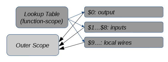
Here is an example function (an arithmetic multiplexer, to be specific).
@function(a_mux,
    @out: 1, @in: 8, /* ... */)
  // $0: output
  // $1 ... $4: data input wires
  // $5 ... $8: selector input wires
  $9 <- @mul($1, $5);
  $10 ... $12 <- @for i @first 2 @last 4
    $(9+i) <- @anon_call(
         $i, $(5+i), $(8+i), /* ... */)
      $4 <- @mul($1, $2);
      $0 <- @add($3, $4);
    @end
  @end
  $0 <- $12;
@end
In its first invocation, all remaps are contiguous, so the only discontiguity is between the input and local ranges.
/* Assume $4 ... $11 are assigned */
$3 <- @call(a_mux, $4 ... $11);
In the second invocation, there are consecutive discontiguities within and around the input and output ranges.
/* Assume $0 ... $20 are assigned */
$22 <- @call(a_mux, $0 ... $2, $9, $5 ... $6, $15, $20)
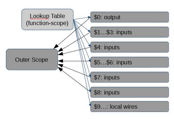
The net effect is that more time is spent remapping small ranges into the lookup table, and that there is a lot of pollution in the table.
What Else is Missing?
In addition to the deficiencies in the wire-numbering system, we believe the following somewhat obvious features should be added to the IR.
- Size-Parameterized Function Gates
-
At the moment a function gate must have a fixed number of input and output wires. As a simple example, consider a function gate that sums all its input wires. To sum 4 wires, 5 wires, or 6 wires one would need different function gates, even though it seems like an obvious enough task for a single function gate to handle.
- Switch Default Case
-
The IR does not allow for programmable behavior if no case is matched within a switch statement. Switches are the only element of the IR that allow for input-dependent control flow; loops and function gates have fixed size, and recursion is strictly forbidden. It makes sense that they be as flexible as possible.
Conclusions
In an early iteration of this article, the conclusion was that many of the criticisms I came up with would be moot if we implemented a two-pass interpreter for the IR. Memory boundaries could then be reconstructed and used to improve performance. Well, as I finish writing this update, said two-pass interpreter, BOLT, is partially implemented, and it will be the subject of a later article. However, in developing BOLT, it became apparent that just having bounds was not the end of the story. Most notably in processing loops, there was no enforcement of the meager bounds that had been reconstructed in the first pass.
Another to-be-written article will discuss what changes Wizkit would like to make in the next IR iteration. Much of the emphasis of the proposed changes will be on making memory boundaries clear to the IR. I think another worthy goal, in the realm of balancing performance and complexity, would be for single-pass interpreters of the next IR to be competitive with multi-pass interpreters for this iteration.